R: Binomial Distribution - UNDER CONSTRUCTION
1. Calculating Exact Binomial Probabilities
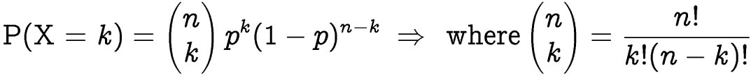
Example: For X~B(10, 0.5), find the P(X = 3)
Example: For X~B(10, 0.5), find the P(X = 3)
R CODE
dbinom(3,10,0.3) # dbinom(k, n, p)
R OUTPUT
[1] 0.2668279
2. Calculating Cumulative Binomial Probabilities
Example: For X~B(10, 0.5), find the P(X ≤ 3)
R CODE
Example: For X~B(10, 0.5), find the P(X ≤ 3)
R CODE
pbinom(3,10,0.3) # pbinom(x, n, p)
R OUTPUT
[1] 0.6496107
3. Simulating Binomial Random Variables
In statistics, one often finds the need to simulate random scenarios that are binomial. To do this, we need to use the rbinom() function. To use the rbinom() function, you need to define three parameters:
EXAMPLE 1:
Let's say you wanted to simulate rolling a dice 5 times, and you wished to count the number of 3's you observe. You could simulate this experiment using the following code:
R CODE
rbinom(1,5,1/6) ### rbinom(number of experiments, number of observations per experiment, probability of success)
R OUTPUT
[1] 2
Conclusion: The above code simulated rolling a die five times. The output of 2 means that there were 2 "successes", or 2 observed 3's as rolling a 3 was labeled as a "success".
Example 2:
Let's say you wanted to simulate a class of 30 students rolling a dice 10 times, and you wished to count the number of 3's you observe for each student. You could simulate this experiment using the following code:
R CODE
Let's say you wanted to simulate a class of 30 students rolling a dice 10 times, and you wished to count the number of 3's you observe for each student. You could simulate this experiment using the following code:
R CODE
rbinom(30,10,1/6) ### rbinom(number of experiments, number of observations per experiment, probability of success)
R OUTPUT
[1] 1 3 1 3 2 0 0 2 2 1 1 0 1 2 1 1 5 3 3 0 1 2 3 1 3 0 1 3 4 0
Conclusion: The above output shows the number of "successes" recorded by each of the 30 students. For example, each student rolled a die 10 times and recorded the number of 3's they observed. The first student recorded only one 3, while the second student recorded three 3's.
Example 3:
Let's say you wanted to simulate a class of 30 students rolling a dice 10 times, and you wished to count the number of 3's you observe for each student. You could simulate this experiment, then create a table using the table() function to summarize your results using the following code:
R CODE
Let's say you wanted to simulate a class of 30 students rolling a dice 10 times, and you wished to count the number of 3's you observe for each student. You could simulate this experiment, then create a table using the table() function to summarize your results using the following code:
R CODE
s=rbinom(30,10,1/6) ### rbinom(number of experiments, number of observations per experiment, probability of success)
table(s)
R OUTPUT
0 1 2 3
8 11 4 7
Conclusion: The R output creates a simple table showing, for instance, of the 30 students who rolled their dice 10 times, 8 of them observed no "successes" or no 3's, while 11 students observed exactly one three.
Example 4:
Let's say you wanted to simulate a class of 1000 students rolling a dice 10 times, and you wished to count the number of 3's you observe for each student. You could simulate this experiment using the following code:
R CODE
Let's say you wanted to simulate a class of 1000 students rolling a dice 10 times, and you wished to count the number of 3's you observe for each student. You could simulate this experiment using the following code:
R CODE
|
### To simulate one random Bernoulli trial, we use the binomial
### distribution and set n=1. e=1 # simulate 1 experiment only n=1 # define 1 observation for this 1 experiment p=.5 # define the probability of success rbinom(e,n,p) ### conduct the random simulation e=10 # simulate 10 independent experiments n=5 # define 1 observation for each of the 10 independent experiments rbinom(e,n,p) ### conduct the 10 random simulations n=100000 ### number of binomial simulations x=rbinom(n, 10, 0.5) table(x) ### table with frequency t=(table(x)/n)*100 ### Create a distribution table with proportions t plot(t, ylab="Probability", main="n=10, p=0.5") ### plot table t ### The binomial distribution requires two parameters to define the ### distribution. The two parameters are n (the number of Bernoulli ### trials) and p (the probability of success). ### To generate binomial numbers, we simply change the value of n from ### 1 to the desired number of trials. For example, with 10 trials: n=10 ### Define n, the number of trials p=0.5 ### Define p, the probability of success x=0:n ### Creates a sequence 0, 1, 2, ..., 10 ### dbinom function calculates the exact probability ### of success for every x, 1:10 prob=dbinom(x,size=n,prob=p)*100 table=rbind(x, prob) ### Creates a table by combing rows x & prob round(table, 1) ### Round numbers in table plot(x,prob, xlim=c(-1,n+1),type="h", lwd=2,col="blue", ylab="Probability",main="n=10, p=0.5") ### The function pbinom is useful for summing consecutive binomial ### probabilities. With n = 10 and p = 0.3, here are some example ### calculations. For example: #### Example A) P(X ≤ 3) pbinom(3,10,0.3) ### pbinom(x, n, p) ### OR sum(dbinom(0 : 3, 10, 0.3)) ### OR ### P(X ≤ y) = 0.6496 => To find y, use the qbinom function qbinom(0.6496, 10, 0.3) ########################### ### Example B) P(X ≥ 4) = 1 − P(X ≤ 3) 1-pbinom(3, 10, 0.3) ### OR sum(dbinom(4 : 10, 10, 0.3)) ############################ ### Example C) P(2 ≤ X ≤ 4) = P(X ≤ 4) − P(X ≤ 1) pbinom(4,10,0.3) - pbinom(1,10,0.3) ### OR sum(dbinom(2:4, 10, 0.3)) ### Graphically represent P(2 ≤ X ≤ 4) n=10 ### Define n x=2:4 ### Define P(2 ≤ X ≤ 4) p=0.3 ### Define p, the probability of success #### The following code will create a nice graph to represent #### the P(2 ≤ X ≤ 4) y=0:n; y=y[-(x+1)] prob=dbinom(x,size=n,prob=p) plot(x,prob,type="h", xlim=c(-1,n+1), ylim=c(0, max(prob)+.05),lwd=2,col="green", ylab="Probability", main="Binomial Distribution") prob=dbinom(y,size=n,prob=p) lines(y,prob, type="h", lwd=2,col="red") |
> ### To simulate one random Bernoulli trial, we use the binomial
> ### distribution and set n=1. > e=1 # simulate 1 experiment only > n=1 # define 1 observation for this 1 experiment > p=.5 # define the probability of success > rbinom(e,n,p) ### conduct the random simulation [1] 0 > > e=10 # simulate 10 independent experiments > n=5 # define 1 observation for each of the 10 independent experiments > rbinom(e,n,p) ### conduct the 10 random simulations [1] 3 2 3 4 2 2 0 2 4 2 > > n=100000 ### number of binomial simulations > x=rbinom(n, 10, 0.5) > table(x) ### table with frequency x 0 1 2 3 4 5 6 7 8 9 10 117 949 4308 11680 20536 24621 20475 11791 4453 950 120 > > t=(table(x)/n)*100 ### Create a distribution table with proportions > t x 0 1 2 3 4 5 6 7 8 9 10 0.12 0.95 4.31 11.68 20.54 24.62 20.48 11.79 4.45 0.95 0.12 > > plot(t, ylab="Probability", main="n=10, p=0.5") ### plot table t 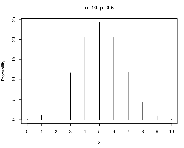 > n=10 ### Define n, the number of trials > p=0.5 ### Define p, the probability of success > x=0:n ### Creates a sequence 0, 1, 2, ..., 10 > > ### dbinom function calculates the exact probability > ### of success for every x, 1:10 > prob=dbinom(x,size=n,prob=p)*100 > > table=rbind(x, prob) ### Creates a table by combing rows x & prob > round(table, 1) ### Round numbers in table [,1] [,2] [,3] [,4] [,5] [,6] [,7] [,8] [,9] [,10] [,11] x 0.0 1 2.0 3.0 4.0 5.0 6.0 7.0 8.0 9 10.0 prob 0.1 1 4.4 11.7 20.5 24.6 20.5 11.7 4.4 1 0.1 > > plot(x,prob, xlim=c(-1,n+1),, lwd=2,col="blue", + ylab="Probability",main="n=10, p=0.5") 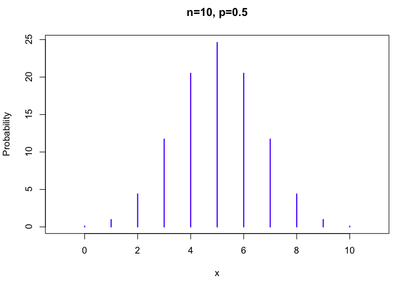 > ### The function pbinom is useful for summing consecutive binomial > ### probabilities. With n = 10 and p = 0.3, here are some example > ### calculations. For example: > > #### Example A) P(X ≤ 3) > pbinom(3,10,0.3) ### pbinom(x, n, p) [1] 0.6496107 > > ### OR > > sum(dbinom(0 : 3, 10, 0.3)) [1] 0.6496107 > > ### OR > > ### P(X ≤ y) = 0.6496 => To find y, use the qbinom function > qbinom(0.6496, 10, 0.3) [1] 3 > > ########################### > ### Example B) P(X ≥ 4) = 1 − P(X ≤ 3) > 1-pbinom(3, 10, 0.3) [1] 0.3503893 > > ### OR > > sum(dbinom(4 : 10, 10, 0.3)) [1] 0.3503893 > > ############################ > ### Example C) P(2 ≤ X ≤ 4) = P(X ≤ 4) − P(X ≤ 1) > pbinom(4,10,0.3) - pbinom(1,10,0.3) [1] 0.7004233 > > ### OR > > sum(dbinom(2:4, 10, 0.3)) [1] 0.7004233 > > ### Graphically represent P(2 ≤ X ≤ 4) > n=10 ### Define n > x=2:4 ### Define P(2 ≤ X ≤ 4) > p=0.3 ### Define p, the probability of success > > > #### The following code will create a nice graph to represent > #### the P(2 ≤ X ≤ 4) > y=0:n; y=y[-(x+1)] > prob=dbinom(x,size=n,prob=p) > plot(x,prob,, xlim=c(-1,n+1), ylim=c(0, max(prob)+.05),lwd=2,col="green", ylab="Probability", main="Binomial Distribution") > > prob=dbinom(y,size=n,prob=p) > lines(y,prob, , lwd=2,col="red") 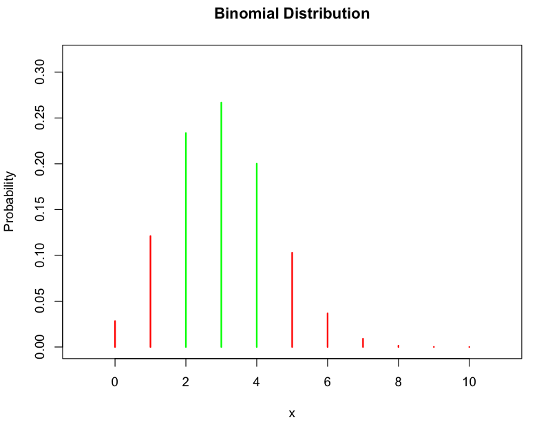 |

This work is licensed under a Creative Commons Attribution-NonCommercial-ShareAlike 3.0 Unported License.
