R: Linear Regression
Code Only
|
Code with Rweb Output
|
|
The following code refers to the Bangladesh Fossil Fuel emission data.
The dataset URL is as follows: http://www.stats4stem.org/uploads/1/7/6/7/1767713/bangledeshh.txt #### CODE STARTS HERE
#### tff = Total Fossil-Fuel Emissions #### gf = Emissions from Gas Fuels plot(tff, gf) # Create a scatterplot # Create a linear model between tff and gf # lm(RESPONSE VARIABLE~EXPLANATORY VARIABLE) or lm(y~x) model=lm(gf~tff) summary(model) ### Reports complete output for the linear model abline(model) ### adds the regression line to the scatterplot ### List outputs that are stored under model that you can call on names(model) ### To call any of the stored names, use ### model$specific.stored.name residuals=model$residuals residuals ### Plot Residuals against x plot(tff,residuals, main="Residual Plot", xlab="Total Fossil Fuel Emissions", ylab="Residuals") ### Add horizontal line at 0 to improve readability of graph abline(h=0) qqnorm(residuals, ylab="Standardized Residuals", xlab="Normal Scores", main="Analysis - Check Assumption of Normality for Residuals") qqline(residuals) |
> #### CODE STARTS HERE
> #### tff = Total Fossil-Fuel Emissions > #### gf = Emissions from Gas Fuels Rweb > > plot(tff, gf) # Create a scatterplot 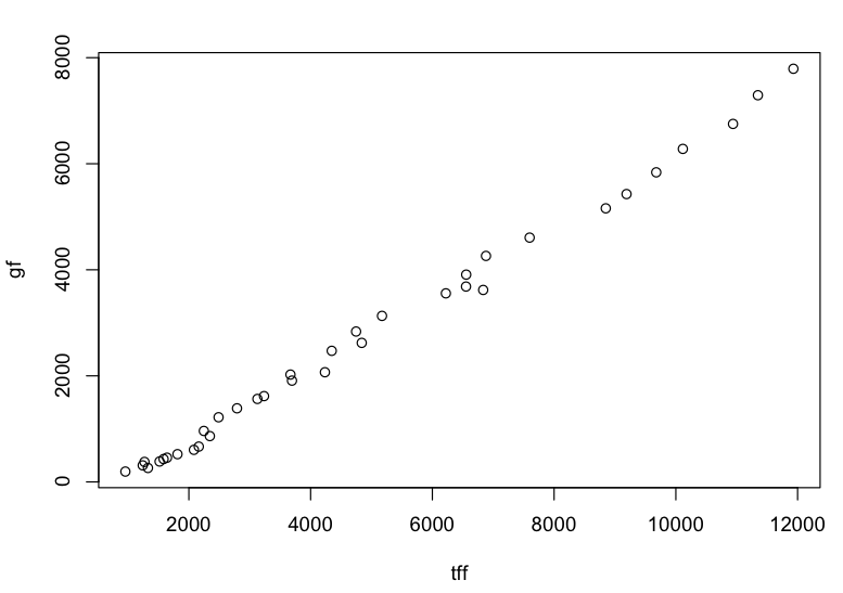 > # Create a linear model between tff and gf
> # lm(RESPONSE VARIABLE~EXPLANATORY VARIABLE) or lm(y~x) > model=lm(gf~tff) > > summary(model) ### Reports complete output for the linear model Call: lm(formula = gf ~ tff) Residuals: Min 1Q Median 3Q Max -412.98 -103.26 14.81 125.38 295.93 Coefficients: Estimate Std. Error t value Pr(>|t|) (Intercept) -6.106e+02 4.775e+01 -12.79 1.52e-14 *** tff 6.794e-01 8.159e-03 83.27 < 2e-16 *** --- Signif. codes: 0 ‘***’ 0.001 ‘**’ 0.01 ‘*’ 0.05 ‘.’ 0.1 ‘ ’ 1 Residual standard error: 159.1 on 34 degrees of freedom Multiple R-squared: 0.9951, Adjusted R-squared: 0.995 F-statistic: 6934 on 1 and 34 DF, p-value: < 2.2e-16 > abline(model) ### adds the regression line to the scatterplot 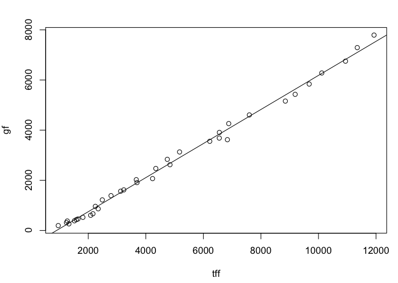 > ### List outputs that are stored under model that you can call on > names(model) [1] "coefficients" "residuals" "effects" "rank" [5] "fitted.values" "assign" "qr" "df.residual" [9] "xlevels" "call" "terms" "model" > > ### To call any of the stored names, use > ### model$specific.stored.name > residuals=model$residuals > > residuals 1 2 3 4 5 6 155.39213 78.77021 124.06833 -28.65606 -36.41672 -35.25548 7 8 9 10 11 12 -47.30049 -98.15302 -199.58432 -192.93433 -118.58061 45.67753 13 14 15 16 17 18 139.26874 102.41806 51.82737 30.77548 10.94227 141.92665 19 20 21 22 23 24 -198.59970 129.31028 -55.62168 221.56021 227.14639 -60.51817 25 26 27 28 29 30 -157.39136 -412.97516 65.57052 197.77358 55.66158 -242.23676 31 32 33 34 35 36 -204.90370 -126.43879 18.67426 -70.13089 193.00467 295.92894 > > ### Plot Residuals against x > plot(tff,residuals, + main="Residual Plot", + xlab="Total Fossil Fuel Emissions", + ylab="Residuals") 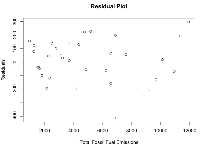 > ### Add horizontal line at 0 to improve readability of graph > abline(h=0) 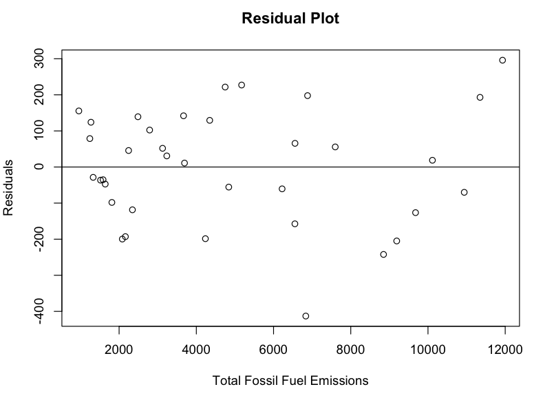 ### Analyze assumption of normality of residualsqqnorm(residuals, ylab="Standardized Residuals", xlab="Normal Scores", main="Analysis - Check Assumption of Normality for Residuals") qqline(residuals) 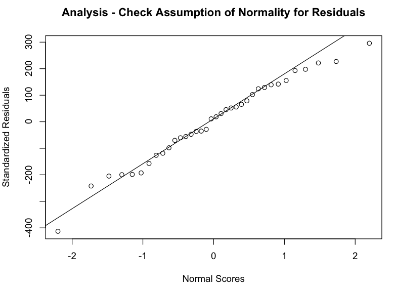 |
Rweb Work Area
DATASET URL:
http://www.stats4stem.org/uploads/1/7/6/7/1767713/bangledeshh.txt
VARIABLES: "year" "tff" "gf" "lf" "sf" "gfl" "cp" "pce.rate" "bf"
http://www.stats4stem.org/uploads/1/7/6/7/1767713/bangledeshh.txt
VARIABLES: "year" "tff" "gf" "lf" "sf" "gfl" "cp" "pce.rate" "bf"
